Difference-in-Differences in 2020
Common Pitfalls and How to Avoid Them
Andrew Baker
Stanford University
2020-09-21
Outline of Talk
Overview of DiD
Problems with Staggered DiD
Simulation Results
Some Alternative Methods
Application
Difference-in-Differences
Think Card and Krueger minimum wage study comparing NJ and PA.
2 units and 2 time periods.
1 unit (T) is treated, and receives treatment in the second period. The control unit (C) is never treated.
Difference-in-Differences
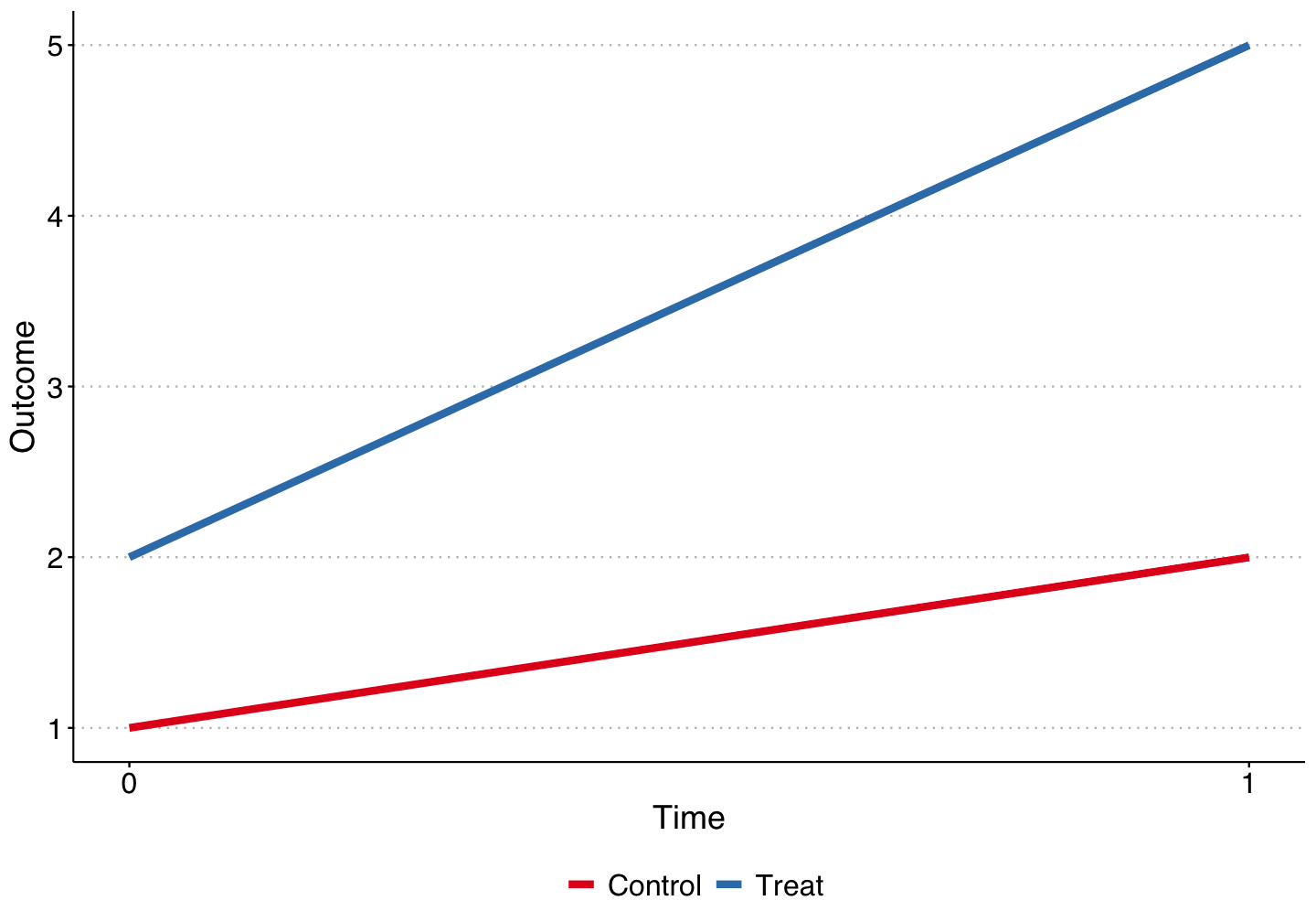
Difference-in-Differences
Building upon Angrist & Pischke (2008, p. 228)Angrist & Pischke (2008, p. 228) we can think of these simple 2x2 DiDs as a fixed effects estimator.
Potential Outcomes
- Y1i,tY1i,t = value of dependent variable for unit ii in period tt with treatment.
- Y0i,tY0i,t = value of dependent variable for unit ii in period tt without treatment.
The expected outcome is a linear function of unit and time fixed effects: E[Y0i,t]=αi+αtE[Y0i,t]=αi+αt E[Y1i,t]=αi+αt+δDstE[Y1i,t]=αi+αt+δDst
- Goal of DiD is to get an unbiased estimate of the treatment effect δδ.
Difference-in-Differences as Solving System of Equations for Unknown Variable
Difference in expectations for the control unit times t = 1 and t = 0: E[Y0C,1]=α1+αCE[Y0C,0]=α0+αCE[Y0C,1]−E[Y0C,0]=α1−α0
Now do the same thing for the treated unit: E[Y1T,1]=α1+αT+δE[Y1T,0]=α0+αTE[Y1T,1]−E[Y1T,0]=α1−α0+δ
- If we assume the linear structure of DiD, then unbiased estimate of δ is:
δ=(E[Y1T,1]−E[Y1T,0])−(E[Y0C,1]−E[Y0C,0])
Two-Way Differencing
Regression DiD
The DiD can be estimated through linear regression of the form:
yit=α+β1TREATi+β2POSTt+δ(TREATi⋅POSTt)+ϵit
The coefficients from the regression estimate in (1) recover the same parameters as the double-differencing performed above: α=E[yit|i=C,t=0]=α0+αCβ1=E[yit|i=T,t=0]−E[yit|i=C,t=0]=(α0+αT)−(α0+αC)=αT−αCβ2=E[yit|i=C,t=1]−E[yit|i=C,t=0]=(α1+αC)−(α0+αC)=α1−α0δ=(E[yit|i=T,t=1]−E[yit|i=T,t=0])−(E[yit|i=C,t=1]−E[yit|i=Ct=0])=δ
Regression DiD - The Workhorse Model
Advantage of regression DiD - it provides both estimates of δ and standard errors for the estimates.
Angrist & Pischke (2008):
- "It's also easy to add additional (units) or periods to the regression setup... [and] it's easy to add additional covariates."
Two-way fixed effects estimator: yit=αi+αt+δDDDit+ϵit
αi and αt are unit and time fixed effects, Dit is the unit-time indicator for treatment.
TREATi and POSTt now subsumed by the fixed effects.
can be easily modified to include covariate matrix Xit, time trends, dynamic treatment effects estimation, etc.
Where It Goes Wrong
Developed literature now on the issues with TWFE DiD with "staggered treatment timing" (Abraham and Sun (2018), Borusyak and Jaravel (2018), Callaway and Sant'Anna (2019), Goodman-Bacon (2019), Strezhnev (2018), Athey and Imbens (2018))
- Different units receive treatment at different periods in time.
Probably the most common use of DiD today. If done right can increase amount of cross-sectional variation.
Without digging into the literature:
δDD with staggered treatment timing is a weighted average of many different treatment effects.
We know little about how it measures when treatment timing varies, how it compares means across groups, or why different specifications change estimates.
The weights are often negative and non-intuitive.
Bias with TWFE - Goodman-Bacon (2019)
- Goodman-Bacon (2019) provides a clear graphical intuition for the bias. Assume three treatment groups - never treated units (U), early treated units (k), and later treated units (l).

Bias with TWFE - Goodman-Bacon (2019)
- Goodman-Bacon (2019) shows that we can form four different 2x2 groups in this setting, where the effect can be estimated using the simple regression DiD in each group:
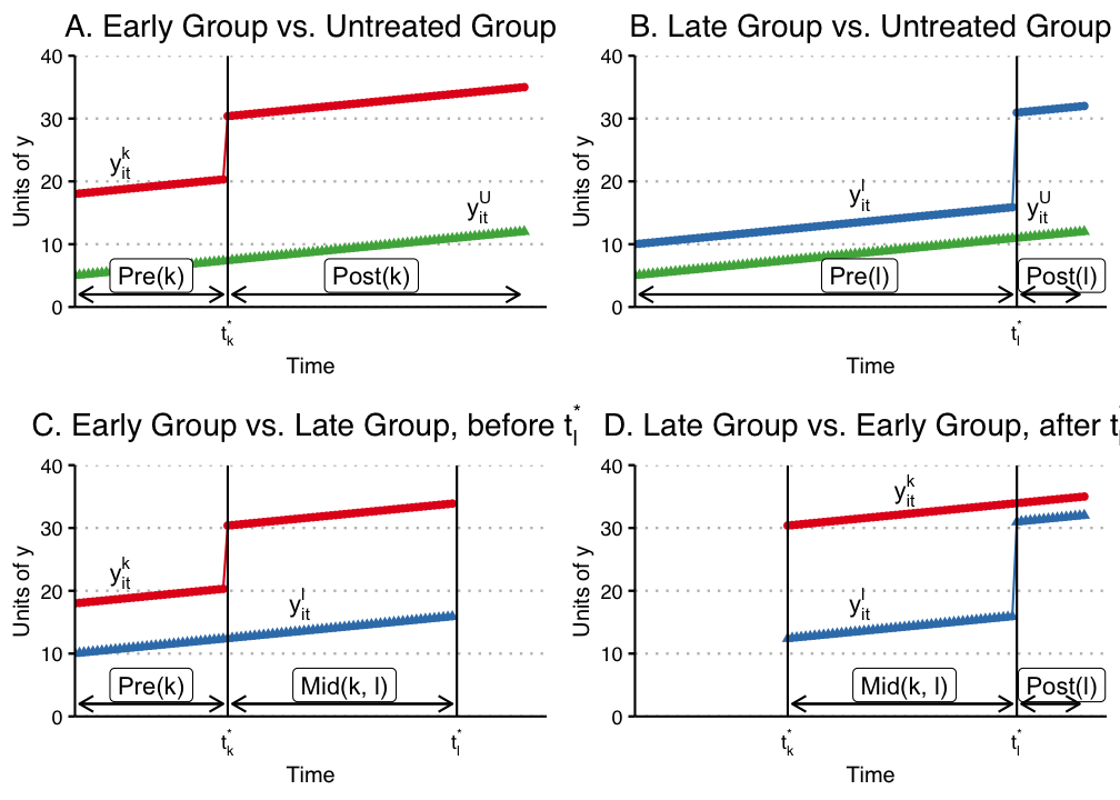
Bias with TWFE - Goodman-Bacon (2019)
Important Insights
δDD is just the weighted average of the four 2x2 treatment effects. The weights are a function of the size of the subsample, relative size of treatment and control units, and the timing of treatment in the sub sample.
Already-treated units act as controls even though they are treated.
Given the weighting function, panel length alone can change the DiD estimates substantially, even when each δDD does not change.
Groups treated closer to middle of panel receive higher weights than those treated earlier or later.
Simulation Exercise
Can show how easily δDD goes awry up through a simulation exercise.
Assume we're modeling outcome variable yit on balanced panel with T=36 years from 1980 to 2015 with 1000 firms i.
Time-invariant unit effects and time-varying year effects drawn from ∼N(0,122).
Firms are incorporate in of 50 randomly drawn states, and states are randomly assigned into three treatment groups Gg∈{1989,1998,2006}.
Simulation Exercise
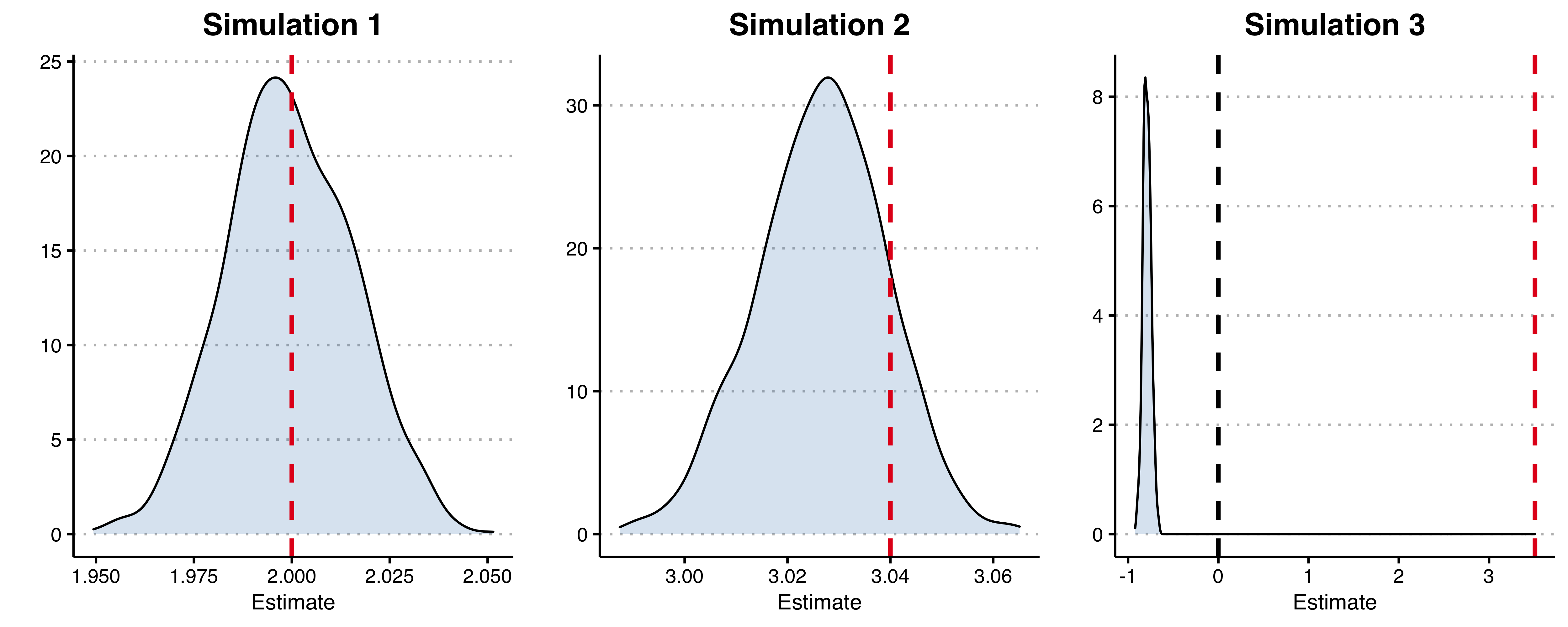
Model the treatment effect process in three ways
Only one treatment period (1998) and one treated group, with constant additive treatment effects.
Allow for staggered treatment timing but with constant additive effects. Simulated treatment effects τ are all positive in expectation but decrease over time ($\tau{G1989} = 5, \tau{G1998} = 3, \tau_{G2007} = 1$).
Allow for both staggered treatment timing and change-in-trend "dynamic" treatment effects. Instead of a constant τ for each group, τi is the yearly increase in outcome variable that compounds over time. Here τi,G1989=0.5,τi,G1998=0.3, and τi,G2007=0.1.
Simulation Exercise

Simulation Exercise
- With the simulated data we estimate TWFE DiD using MLE on:
yit=αi+αt+δDDDit+ϵit
- Simple regression model with unit and time fixed effects.
- For each of the three simulated datasets we run a Monte Carlo simulation where we create the datasets 1,000 times and plot the distribution of ^δDD.
- Bias is deviation from true underlying treatment effect.
Simulation Exercise
Goodman-Bacon Decomposition for Simulation 3
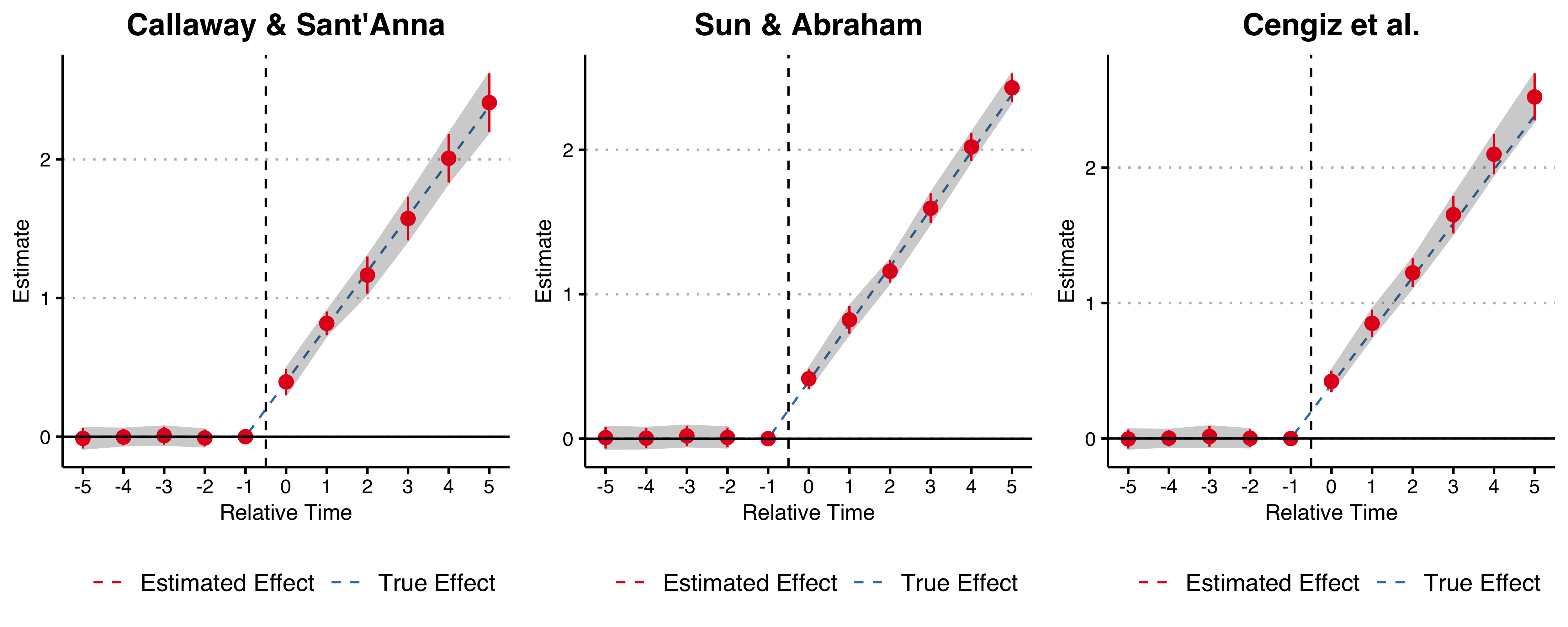
Callaway & Sant'Anna
- Inverse propensity weighted long-difference in cohort-specific average treatment effects between treated and untreated units for a given treatment cohort.
ATT(g,t)=E[(GgE[Gg]−pg(X)C1−pg(X)E[pg(X)C1−pg(X)])(Yt−Tg−1)]
Abraham and Sun
A relatively straightforward extension of the standard event-study TWFE model:
yit=αi+αt+∑e∑l≠−1δel(1{Ei=e}⋅Dlit)+ϵit
You saturate the relative time indicators (i.e. t = -2, -1, ...) with indicators for the treatment initiation year group, and aggregate to overall aggregate relative time indicators by cohort size.
In the case of no covariates, this gives you the same estimate as Callaway & Sant'Anna if you fully saturate the model with time indicators (leaving only two relative year identifiers missing).
The authors don't claim that it can be used with covariates, but it seemingly follows if we think it is okay with normal TWFE DiD.
Stacked Regression
Similar to the standard TWFE DiD, but we ensure that no previously treated units enter as controls by trimming the sample.
For each treatment cohort Gg, get all treated units, and all units that are not treated by year g+k where g is the treatment year and k is the outer most relative year that you want to test (e.g. if you do an event study plot from -5 to 5, k would equal 5).
Keep only observations within years g−k and g+k for each cohort-specific dataset, and then stack them in relative time.
Run the same TWFE estimates as in standard DiD, but include interactions for the cohort-specific dataset with all of the fixed effects, controls, and clusters.
Simulations - Remedies
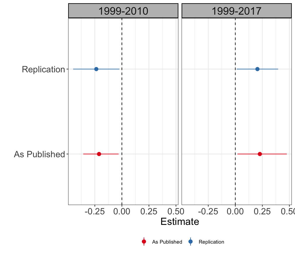
Application - Medical Marijuana Laws and Opioid Overdose Deaths
Bachhuber et al. 2014 found, using a staggered DiD, that states with medical cannabis laws experienced a slower increase in opioid overdose mortality from 1999-2010.
Shover et al. 2020 extend the data sample from 2010 to 2017, a period during which 32 extra states passed MML laws.
Not only do the results go away, but the sign flips; MML laws are associated with higher opioid overdose mortality rates.
Authors don't call it difference-in-differences, but it uses TWFE with a binary indicator variable (thus is effectively DiD).
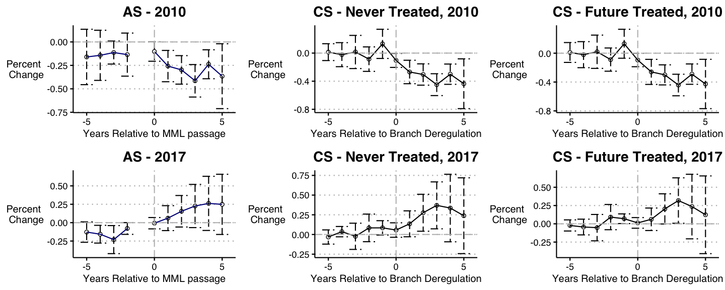
Replication of MML
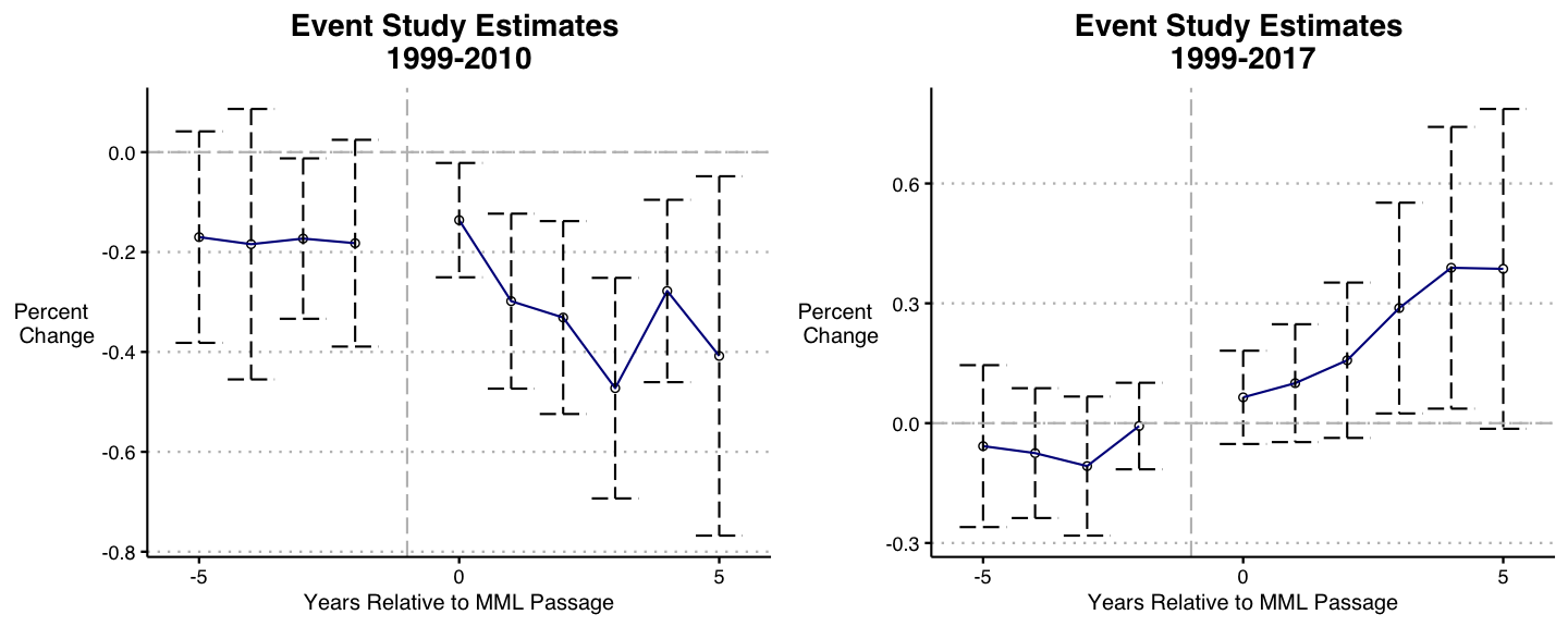
Event Study Estimates
Little evidence covariates matter here, so estimate standard DiD with no controls over the two periods:
yit=αi+αt+k∗∑k=k∗δkDit+ϵit
where αi and αt are state and year fixed effects respectively, and δk are the coefficients on the lead/lag indicators for years around treatment.
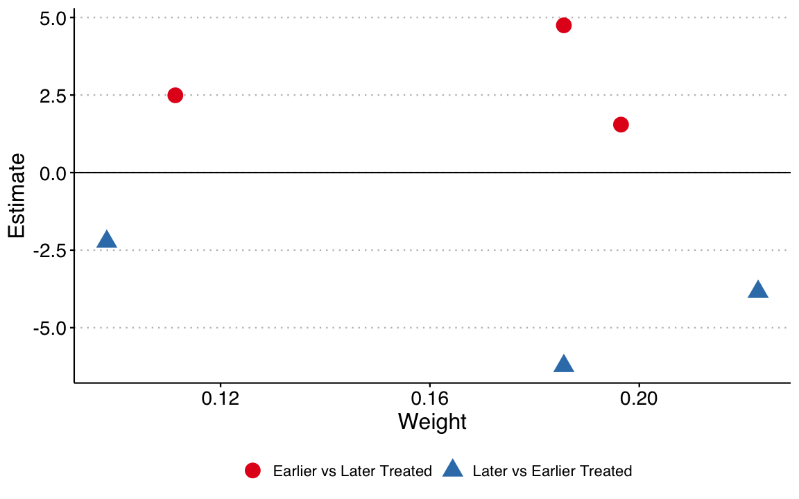
Goodman-Bacon Decomposition
1999-2010 |
1999-2017 |
|||||
|---|---|---|---|---|---|---|
| Type | Average Estimate | Number of 2x2 Comparisons | Total Weight | Average Estimate | Number of 2x2 Comparisons | Total Weight |
| Earlier vs Later Treated | -0.11 | 21 | 0.04 | -0.16 | 91 | 0.38 |
| Later vs Earlier Treated | 0.09 | 28 | 0.16 | 0.32 | 105 | 0.42 |
| Treated vs Untreated | -0.25 | 7 | 0.79 | 0.44 | 14 | 0.20 |
Remedies
Takeaways
DiDs are a powerful tool and we are going to keep using them.
But we should make sure we understand what we're doing! DiD is a comparison of means and at a minimum we should know which means we're comparing.
Multiple new methods have been proposed, all of which ensure that you aren't using prior treated units as controls.
You should probably tailor your selection of method to your data structure: they use and discard different amount of control units and depending on your setting this might matter.
Unclear what's going on with MMLs and opioid mortality rates, but very unlikely that the results in the first published paper is robust.