How To Create Relative Time Indicators
In this memo we will test empirically whether there are issues with the event-study DiD even if the dynamic treatment effects are constant across cohorts. To do this I will conduct a similar simulation to the one shown in my slides.
The data generating process is \[y_{it} = \alpha_i + \alpha_t + \tau_{it} + \epsilon_{it}\]
where \(\alpha_i\) are unit fixed effects drawn from \(\sim N(0, 1)\), \(\alpha_t\) are period fixed effects, also drawn from \(\sim N(0, 1)\), and the white-noise error term \(\epsilon_{it}\) is drawn from \(\sim N\left(0, \left(\frac{1}{2}\right)^2\right)\).
We will consider a staggered treatment design, where forty states are randomly assigned into four treatment cohorts of size 250 depending on the year of treatment assignment (1986, 1992, 1998, and 2004). There 1000 units \(i\) in are sample are randomly assigned to one of the 40 states. For every unit incorporated in a treated state, we pull a unit-specific treatment effect from \(\mu_i \sim N(0.3, (1/5)^2)\), and the cumulated treatment effect \(\tau_{it}\) is \(\mu_i \times (year - \tau_g + 1)\) where \(\tau_g\) is the treatment year for the state of incorporation. We then estimate the average treatment effect as \(\hat{\delta}\) from:
\[y_{it} = \hat{\alpha_i} + \hat{\alpha_t} + \hat{\delta} D_{it}\]
where with \(D_{it}\) being an indicator for being incorporated in a state on or after it’s treatment assignment year \(\tau_g\). We hope that \(\hat{\delta}\) is an unbiased estimate of the average treatment effect. Because DiD with a binary treatment indicator variable captures the difference in the average post-treatment outcomes to the average pre-treatment outcomes, we can analytically derive the expected average treatment effect.
Because this uses random number generation for the simulated effects, I run the simulation 1000 times and plot the distribution of the treatment effects. The red line indicates the true treatment effects derived above.
First, let’s visualize the data for one simulation so we’re all on the same page with the DGP.
library(tidyverse)
library(lfe)
library(ggthemes)
library(fastDummies)
theme_set(theme_clean() + theme(plot.background = element_blank()))
select <- dplyr::select
set.seed(20200403)
## Generate data - 250 firms are treated every period, with the treatment effect still = 0.3 on average
make_data <- function(...) {
# Fixed Effects ------------------------------------------------
# unit fixed effects
unit <- tibble(
unit = 1:1000,
unit_fe = rnorm(1000, 0, 1),
# generate state
state = sample(1:40, 1000, replace = TRUE),
# generate treatment effect
mu = rnorm(1000, 0.3, 0.2))
# year fixed effects
year <- tibble(
year = 1980:2010,
year_fe = rnorm(31, 0, 1))
# Trend Break -------------------------------------------------------------
# Put the states into treatment groups
treat_taus <- tibble(
# sample the states randomly
state = sample(1:40, 40, replace = FALSE),
# place the randomly sampled states into five treatment groups G_g
cohort_year = sort(rep(c(1986, 1992, 1998, 2004), 10)))
# make main dataset
# full interaction of unit X year
expand_grid(unit = 1:1000, year = 1980:2010) %>%
left_join(., unit) %>%
left_join(., year) %>%
left_join(., treat_taus) %>%
# make error term and get treatment indicators and treatment effects
mutate(error = rnorm(31000, 0, 0.5),
treat = ifelse(year >= cohort_year, 1, 0),
tau = ifelse(treat == 1, mu, 0)) %>%
# calculate cumulative treatment effects
group_by(unit) %>%
mutate(tau_cum = cumsum(tau)) %>%
ungroup() %>%
# calculate the dep variable
mutate(dep_var = unit_fe + year_fe + tau_cum + error)
}
# make data
data <- make_data()
# plot
plot <- data %>%
ggplot(aes(x = year, y = dep_var, group = unit)) +
geom_line(alpha = 1/8, color = "grey") +
geom_line(data = data %>%
group_by(cohort_year, year) %>%
summarize(dep_var = mean(dep_var)),
aes(x = year, y = dep_var, group = factor(cohort_year),
color = factor(cohort_year)),
size = 2) +
labs(x = "", y = "Value") +
geom_vline(xintercept = 1986, color = '#E41A1C', size = 2) +
geom_vline(xintercept = 1992, color = '#377EB8', size = 2) +
geom_vline(xintercept = 1998, color = '#4DAF4A', size = 2) +
geom_vline(xintercept = 2004, color = '#984EA3', size = 2) +
scale_color_brewer(palette = 'Set1') +
theme(legend.position = 'bottom',
legend.title = element_blank(),
axis.title = element_text(size = 14),
axis.text = element_text(size = 12))
plot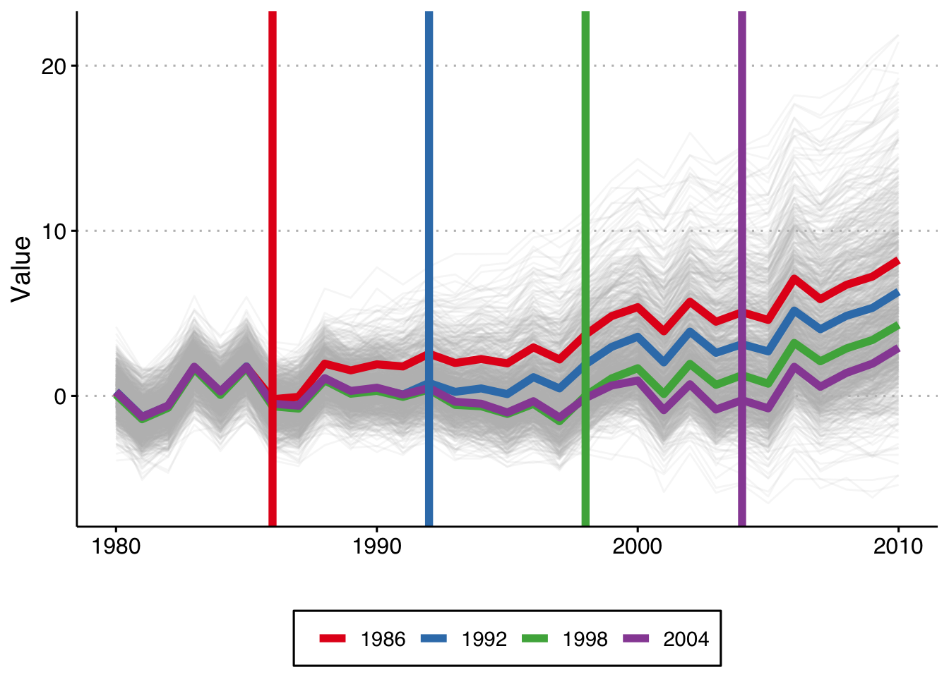 This shows the 1,000 individual values of \(y_{it}\), as well as the average by cohort (in color), and the vertical lines show the period when treatment begins for each cohort. Because this is a trend line shift we see that the earliest treated units end up with the highest value of y, and that the difference grows by gap between treatment years.
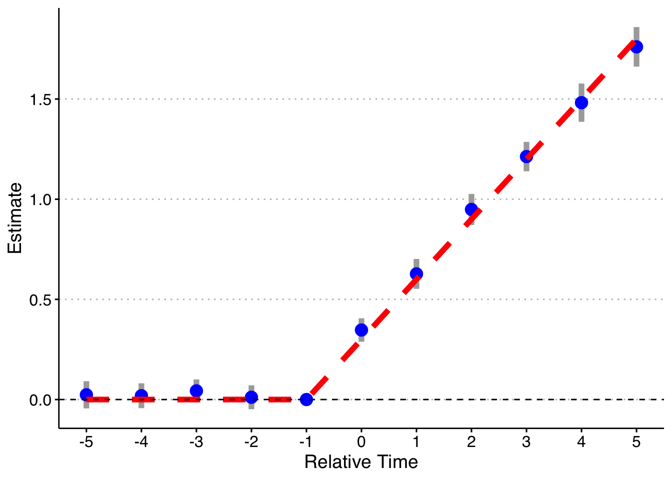
So the first thing we can do is check whether the standard event study method works in this setting (when each cohort gets the same treatment effects but they are dynamic). The first way we will do this is by binning the Pre and Post observations, as is commonly done. That is, we estimate the event-study treatment effects as:
\[y_{it} = \hat{\alpha_i} + \hat{\alpha_t} + \sum_{k \neq -1} \hat{\gamma}_k D_{it}\] where we include lead/lag dummies for the periods from -5 to 5 (omitting t = -1), as well as binned dummies for years less than -5 and years greater than + 5. I will do this 1,000 times and plot the mean and 2 SE confidence interval of the relative time indicator dummies, as well as the true treatment effect below.
# variables we will use
keepvars <- c("`rel_year_-5`",  "`rel_year_-4`",  "`rel_year_-3`",  "`rel_year_-2`",
               "rel_year_0", "rel_year_1", "rel_year_2", "rel_year_3", "rel_year_4", "rel_year_5")

# function to run ES DID
run_ES_DiD <- function(...) {

  # resimulate the data
  data <- make_data()

  # make dummy columns
  data <- data %>%
    # make dummies
    mutate(rel_year = year - cohort_year) %>%
    dummy_cols(select_columns = "rel_year") %>%
    # generate pre and post dummies
     mutate(Pre = ifelse(rel_year < -5, 1, 0),
            Post = ifelse(rel_year > 5, 1, 0))

  # estimate the model
  mod <- felm(dep_var ~ Pre + `rel_year_-5` + `rel_year_-4` + `rel_year_-3` + `rel_year_-2` +
                `rel_year_0` + `rel_year_1` + `rel_year_2` + `rel_year_3` + `rel_year_4` +
                `rel_year_5` + Post | unit + year | 0 | state, data = data, exactDOF = TRUE)

  # grab the obs we need
  broom::tidy(mod) %>%
    filter(term %in% keepvars) %>%
    mutate(t = c(-5:-2, 0:5)) %>%
    select(t, estimate)
}

# run it 1000 times
set.seed(20200403)
data <- map_dfr(1:1000, run_ES_DiD)

data %>%
  group_by(t) %>%
  summarize(avg = mean(estimate),
            sd = sd(estimate),
            lower.ci = avg - 1.96*sd,
            upper.ci = avg + 1.96*sd) %>%
  bind_rows(tibble(t = -1, avg = 0, sd = 0, lower.ci = 0, upper.ci = 0)) %>%
  mutate(true_tau = ifelse(t >= 0, (t + 1)*.3, 0)) %>%
  ggplot(aes(x = t, y = avg)) +
  geom_linerange(aes(ymin = lower.ci, ymax = upper.ci), color = 'darkgrey', size = 2) +
  geom_point(color = 'blue', size = 4) +
  geom_line(aes(x = t, y = true_tau), color = 'red', linetype = "dashed", size = 2) +
  geom_hline(yintercept = 0, linetype = "dashed") +
  scale_x_continuous(breaks = -5:5) +
  labs(x = "Relative Time", y = "Estimate") +
  theme(axis.title = element_text(size = 14),
        axis.text = element_text(size = 12))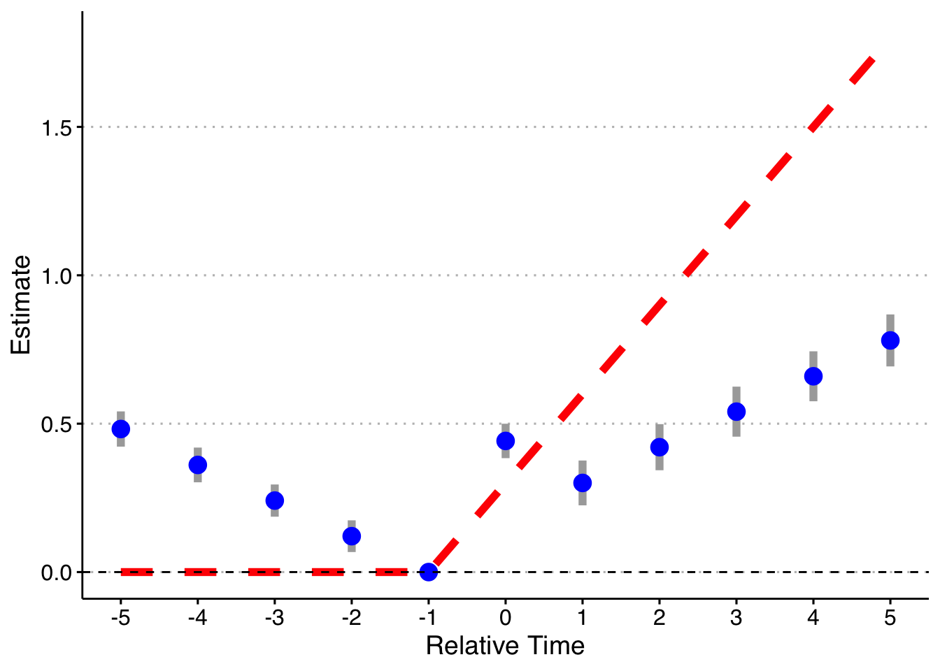
Now, we can drop the indicator for Pre, so that there is only an indicator to control for Post (while still dropping t = -1).
# function to run ES DID
run_ES_DiD <- function(...) {

  # resimulate the data
  data <- make_data()

  # make dummy columns
  data <- data %>%
    # make dummies
    mutate(rel_year = year - cohort_year) %>%
    dummy_cols(select_columns = "rel_year") %>%
    # generate pre and post dummies
     mutate(Pre = ifelse(rel_year < -5, 1, 0),
            Post = ifelse(rel_year > 5, 1, 0))

  # estimate the model
  mod <- felm(dep_var ~ `rel_year_-5` + `rel_year_-4` + `rel_year_-3` + `rel_year_-2` +
                `rel_year_0` + `rel_year_1` + `rel_year_2` + `rel_year_3` + `rel_year_4` + `rel_year_5` +
                Post | unit + year | 0 | state, data = data, exactDOF = TRUE)

  # grab the obs we need
  broom::tidy(mod) %>%
    filter(term %in% keepvars) %>%
    mutate(t = c(-5:-2, 0:5)) %>%
    select(t, estimate)
}

# run it 1000 times
set.seed(20200403)
data <- map_dfr(1:1000, run_ES_DiD)

# plot
data %>%
  group_by(t) %>%
  summarize(avg = mean(estimate),
            sd = sd(estimate),
            lower.ci = avg - 1.96*sd,
            upper.ci = avg + 1.96*sd) %>%
  bind_rows(tibble(t = -1, avg = 0, sd = 0, lower.ci = 0, upper.ci = 0)) %>%
  mutate(true_tau = ifelse(t >= 0, (t + 1)*.3, 0)) %>%
  ggplot(aes(x = t, y = avg)) +
  geom_linerange(aes(ymin = lower.ci, ymax = upper.ci), color = 'darkgrey', size = 2) +
  geom_point(color = 'blue', size = 4) +
  geom_line(aes(x = t, y = true_tau), color = 'red', linetype = "dashed", size = 2) +
  geom_hline(yintercept = 0, linetype = "dashed") +
  scale_x_continuous(breaks = -5:5) +
  labs(x = "Relative Time", y = "Estimate") +
  theme(axis.title = element_text(size = 14),
        axis.text = element_text(size = 12))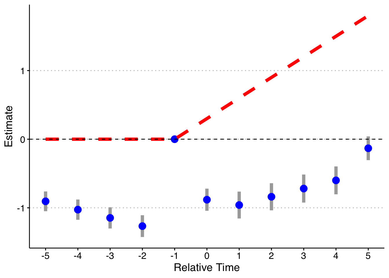
Finally, let’s do the fully saturated model (an indicator for every possible relative year indicator), omitting two periods (the most negative and year t - 1) following Callaway & Sant’Anna and Borusyak & Jaravel.
# function to run ES DID
run_ES_DiD <- function(...) {

  # resimulate the data
  data <- make_data()

  # make dummy columns
  data <- data %>%
    # make relative year indicator
    mutate(rel_year = year - cohort_year)

  # get the minimum relative year - we need this to reindex
  min_year <- min(data$rel_year)

  # reindex the relative years
  data <- data %>%
    mutate(rel_year = rel_year - min_year) %>%
    dummy_cols(select_columns = "rel_year")

  # make regression formula
  indics <- paste("rel_year", (1:max(data$rel_year))[-(-1 - min_year)], sep = "_", collapse = " + ")
  keepvars <- paste("rel_year", c(-5:-2, 0:5) - min_year, sep = "_")
  formula <- as.formula(paste("dep_var ~", indics, "| unit + year | 0 | state"))

  # run mod
  mod <- felm(formula, data = data, exactDOF = TRUE)

  # grab the obs we need
  broom::tidy(mod) %>%
    filter(term %in% keepvars) %>%
    mutate(t = c(-5:-2, 0:5)) %>%
    select(t, estimate)
}

# run it 1000 times
set.seed(20200403)
data <- map_dfr(1:1000, run_ES_DiD)

data %>%
  group_by(t) %>%
  summarize(avg = mean(estimate),
            sd = sd(estimate),
            lower.ci = avg - 1.96*sd,
            upper.ci = avg + 1.96*sd) %>%
  bind_rows(tibble(t = -1, avg = 0, sd = 0, lower.ci = 0, upper.ci = 0)) %>%
  mutate(true_tau = ifelse(t >= 0, (t + 1)*.3, 0)) %>%
  ggplot(aes(x = t, y = avg)) +
  geom_linerange(aes(ymin = lower.ci, ymax = upper.ci), color = 'darkgrey', size = 2) +
  geom_point(color = 'blue', size = 4) +
  geom_line(aes(x = t, y = true_tau), color = 'red', linetype = "dashed", size = 2) +
  geom_hline(yintercept = 0, linetype = "dashed") +
  scale_x_continuous(breaks = -5:5) +
  labs(x = "Relative Time", y = "Estimate") +
  theme(axis.title = element_text(size = 14),
        axis.text = element_text(size = 12))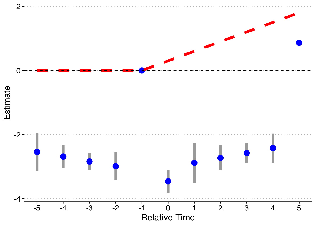
Now, I will trim the sample to end in 2003 (before the last treated cohort). Now 2004 cohorts act as effective controls (I also drop the pre-lags on the 2004 cohort). I will just rely on asymptotic standard errors rather than redoing the simulation 1000 times.
First, the standard way (with bins for both Pre and Post):
keepvars <- c("`rel_year_-5`",  "`rel_year_-4`",  "`rel_year_-3`",  "`rel_year_-2`",
               "rel_year_0", "rel_year_1", "rel_year_2", "rel_year_3", "rel_year_4", "rel_year_5")

# function to run ES DID
run_ES_DiD <- function(...) {

  # resimulate the data
  data <- make_data() %>%
    filter(year <= 2003) %>%
    mutate(cohort_year = ifelse(cohort_year == 2004, 0, cohort_year))

  # make dummy columns
  data <- data %>%
    # make dummies
    mutate(rel_year = year - cohort_year) %>%
    dummy_cols(select_columns = "rel_year") %>%
    # generate pre and post dummies
     mutate(Pre = ifelse(rel_year < -5, 1, 0),
            Post = ifelse(rel_year > 5 & cohort_year != 0, 1, 0))

  # estimate the model
  mod <- felm(dep_var ~ Pre + `rel_year_-5` + `rel_year_-4` + `rel_year_-3` + `rel_year_-2` +
                `rel_year_0` + `rel_year_1` + `rel_year_2` + `rel_year_3` + `rel_year_4` +
                `rel_year_5` + Post | unit + year | 0 | state, data = data, exactDOF = TRUE)

  # grab the obs we need
  broom::tidy(mod, conf.int = TRUE) %>%
    filter(term %in% keepvars) %>%
    mutate(t = c(-5:-2, 0:5)) %>%
    select(t, estimate, conf.low, conf.high)
}

# run it once
set.seed(20200403)
data <- map_dfr(1, run_ES_DiD)

data %>%
  bind_rows(tibble(t = -1, estimate = 0, conf.low = 0, conf.high = 0)) %>%
  mutate(true_tau = ifelse(t >= 0, (t + 1)*.3, 0)) %>%
  ggplot(aes(x = t, y = estimate)) +
  geom_linerange(aes(ymin = conf.low, ymax = conf.high), color = 'darkgrey', size = 2) +
  geom_point(color = 'blue', size = 4) +
  geom_line(aes(x = t, y = true_tau), color = 'red', linetype = "dashed", size = 2) +
  geom_hline(yintercept = 0, linetype = "dashed") +
  scale_x_continuous(breaks = -5:5) +
  labs(x = "Relative Time", y = "Estimate") +
  theme(axis.title = element_text(size = 14),
        axis.text = element_text(size = 12))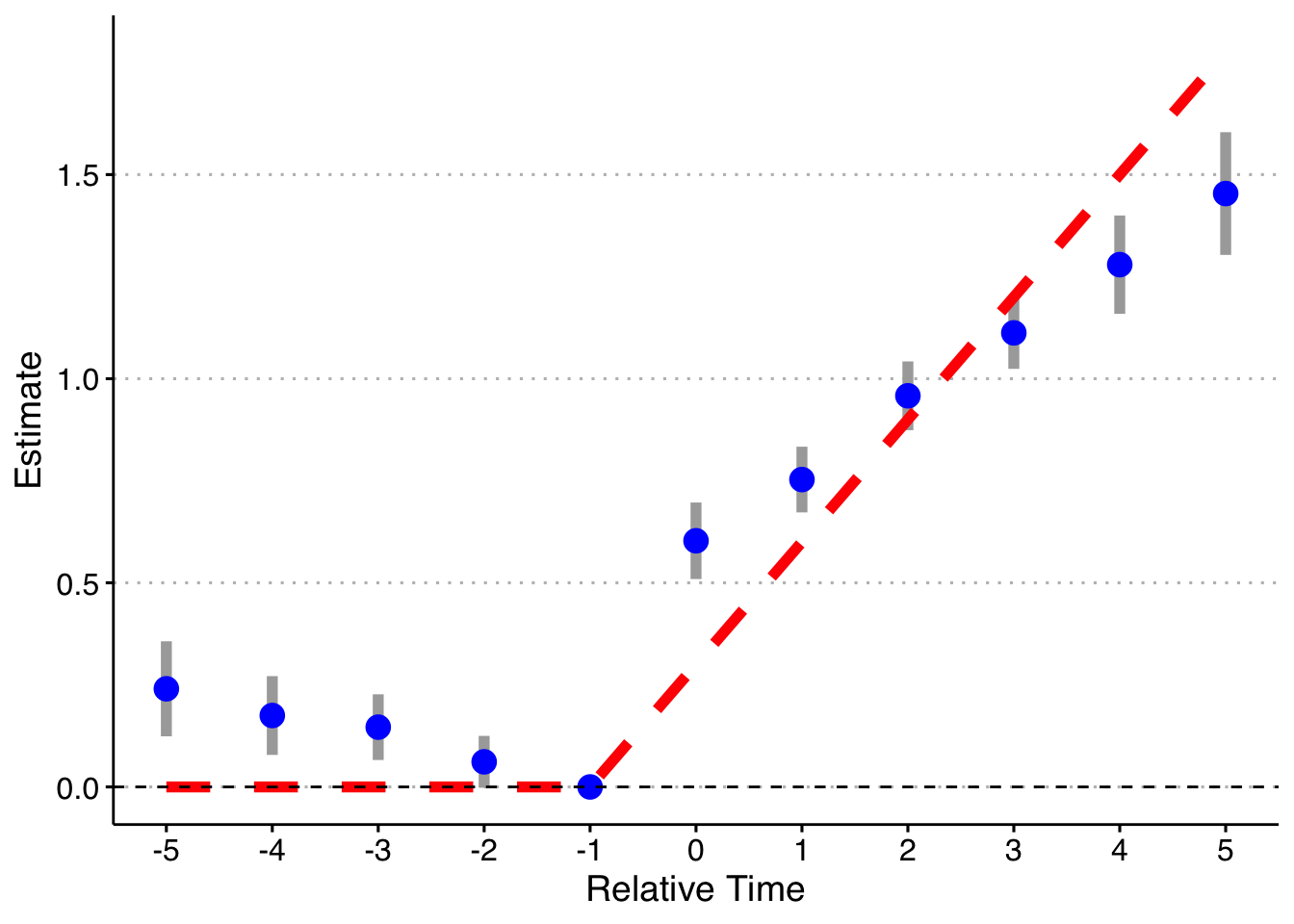
Second, dropping the indicator for Pre, but keeping Post.
keepvars <- c("`rel_year_-5`",  "`rel_year_-4`",  "`rel_year_-3`",  "`rel_year_-2`",
               "rel_year_0", "rel_year_1", "rel_year_2", "rel_year_3", "rel_year_4", "rel_year_5")

# function to run ES DID
run_ES_DiD <- function(...) {

 # resimulate the data
  data <- make_data() %>%
    filter(year <= 2003) %>%
    mutate(cohort_year = ifelse(cohort_year == 2004, 0, cohort_year))

  # make dummy columns
  data <- data %>%
    # make dummies
    mutate(rel_year = year - cohort_year) %>%
    dummy_cols(select_columns = "rel_year") %>%
    # generate pre and post dummies
     mutate(Pre = ifelse(rel_year < -5, 1, 0),
            Post = ifelse(rel_year > 5 & cohort_year != 0, 1, 0))

  # estimate the model
  mod <- felm(dep_var ~ `rel_year_-5` + `rel_year_-4` + `rel_year_-3` + `rel_year_-2` +
                `rel_year_0` + `rel_year_1` + `rel_year_2` + `rel_year_3` + `rel_year_4` +
                `rel_year_5` + Post | unit + year | 0 | state, data = data, exactDOF = TRUE)

  # grab the obs we need
  broom::tidy(mod, conf.int = TRUE) %>%
    filter(term %in% keepvars) %>%
    mutate(t = c(-5:-2, 0:5)) %>%
    select(t, estimate, conf.low, conf.high)
}

# run it once
set.seed(20200403)
data <- map_dfr(1, run_ES_DiD)

data %>%
  bind_rows(tibble(t = -1, estimate = 0, conf.low = 0, conf.high = 0)) %>%
  mutate(true_tau = ifelse(t >= 0, (t + 1)*.3, 0)) %>%
  ggplot(aes(x = t, y = estimate)) +
  geom_linerange(aes(ymin = conf.low, ymax = conf.high), color = 'darkgrey', size = 2) +
  geom_point(color = 'blue', size = 4) +
  geom_line(aes(x = t, y = true_tau), color = 'red', linetype = "dashed", size = 2) +
  geom_hline(yintercept = 0, linetype = "dashed") +
  scale_x_continuous(breaks = -5:5) +
  labs(x = "Relative Time", y = "Estimate") +
  theme(axis.title = element_text(size = 14),
        axis.text = element_text(size = 12))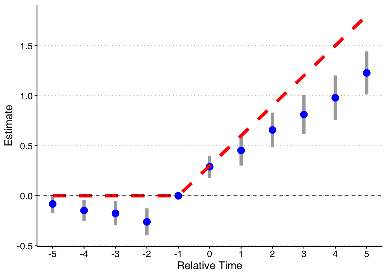
And finally, doing the model fully saturated in relative-year indicators.
# function to run ES DID
run_ES_DiD <- function(...) {

  # resimulate the data
  data <- make_data() %>%
    filter(year <= 2003) %>%
    mutate(cohort_year = ifelse(cohort_year == 2004, 0, cohort_year))

  # make dummy columns
  data <- data %>%
    # make relative year indicator
    mutate(rel_year = year - cohort_year)

  # get the minimum relative year - we need this to reindex
  min_year <- min(data %>% filter(cohort_year != 0) %>% pull(rel_year))

  # reindex the relative years
  data <- data %>%
    mutate(rel_year = rel_year - min_year) %>%
    dummy_cols(select_columns = "rel_year")

  # make regression formula
  indics <- paste("rel_year", (1:max(data %>% filter(cohort_year != 0) %>% pull(rel_year)))[-(-1 - min_year)], sep = "_", collapse = " + ")
  keepvars <- paste("rel_year", c(-5:-2, 0:5) - min_year, sep = "_")
  formula <- as.formula(paste("dep_var ~", indics, "| unit + year | 0 | state"))

  # run mod
  mod <- felm(formula, data = data, exactDOF = TRUE)

  # grab the obs we need
  broom::tidy(mod, conf.int = TRUE) %>%
    filter(term %in% keepvars) %>%
    mutate(t = c(-5:-2, 0:5)) %>%
    select(t, estimate, conf.low, conf.high)
}

# run it 1000 times
set.seed(20200403)
data <- map_dfr(1:1, run_ES_DiD)

data %>%
  bind_rows(tibble(t = -1, estimate = 0, conf.low = 0, conf.high = 0)) %>%
  mutate(true_tau = ifelse(t >= 0, (t + 1)*.3, 0)) %>%
  ggplot(aes(x = t, y = estimate)) +
  geom_linerange(aes(ymin = conf.low, ymax = conf.high), color = 'darkgrey', size = 2) +
  geom_point(color = 'blue', size = 4) +
  geom_line(aes(x = t, y = true_tau), color = 'red', linetype = "dashed", size = 2) +
  geom_hline(yintercept = 0, linetype = "dashed") +
  scale_x_continuous(breaks = -5:5) +
  labs(x = "Relative Time", y = "Estimate") +
  theme(axis.title = element_text(size = 14),
        axis.text = element_text(size = 12))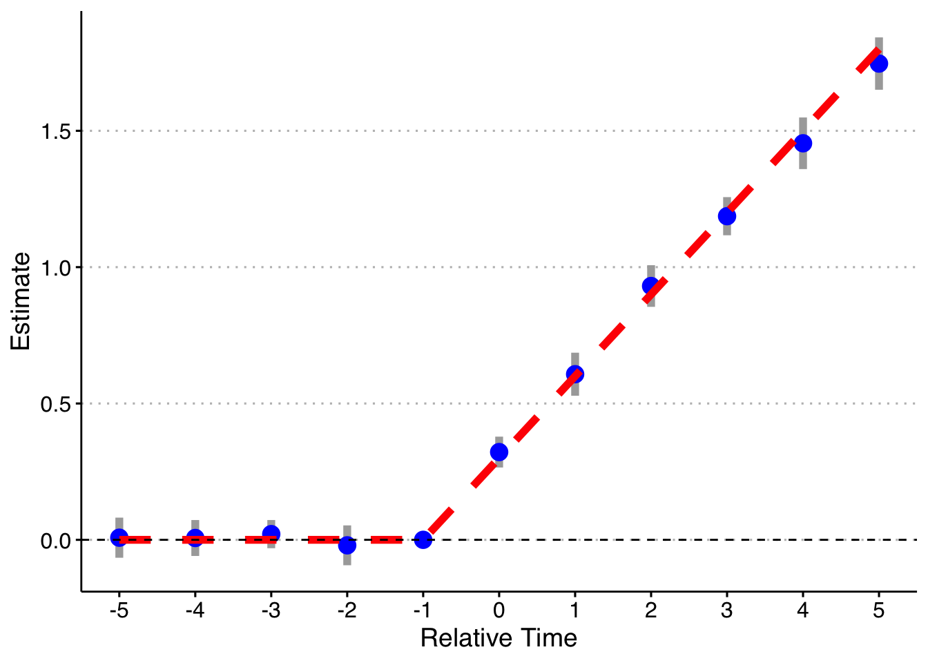
Finally, following a suggestion, let’s look at if we do a binning for the Pre units (relative year less than -5), but fully saturate in the post-treatment units still. Note that it’s impossible to drop two relative time periods here (although you could probably specify the pre-indicator to exclude the most negative relative time and it would likely work). This works! So you can bin if there are no pre-trends, but my strong guess is that you might as well not and do all the relative time indicators.
# function to run ES DID
run_ES_DiD <- function(...) {

  # resimulate the data
  data <- make_data() %>%
    filter(year <= 2003) %>%
    mutate(cohort_year = ifelse(cohort_year == 2004, 0, cohort_year))

  # make dummy columns
  data <- data %>%
    # make relative year indicator
    mutate(rel_year = year - cohort_year)

  # get the minimum relative year - we need this to reindex
  min_year <- min(data %>% filter(cohort_year != 0) %>% pull(rel_year))
  # figure out the less than -5 indicators and the indicator for t = -1
  pre_year <- -5 - min_year
  lag_1 <- -1 - min_year

  # reindex the relative years and make dummies
  data <- data %>%
    mutate(rel_year = rel_year - min_year,
           pre = if_else(rel_year < pre_year, 1, 0)) %>%
    dummy_cols(select_columns = "rel_year")

  # make regression formula
  indics <- paste("rel_year", c(pre_year:(lag_1 - 1),
                                (lag_1 + 1):(max(data %>% filter(cohort_year != 0) %>% pull(rel_year)))),
                  sep = "_", collapse = " + ")
  indics <- paste("pre", indics, sep = " + ")
  keepvars <- paste("rel_year", c(-5:-2, 0:5) - min_year, sep = "_")
  formula <- as.formula(paste("dep_var ~", indics, "| unit + year | 0 | state"))

  # run mod
  mod <- felm(formula, data = data, exactDOF = TRUE)

  # grab the obs we need
  broom::tidy(mod, conf.int = TRUE) %>%
    filter(term %in% keepvars) %>%
    mutate(t = c(-5:-2, 0:5)) %>%
    select(t, estimate, conf.low, conf.high)
}

# run it 1000 times
set.seed(20200403)
data <- map_dfr(1:1, run_ES_DiD)

data %>%
  bind_rows(tibble(t = -1, estimate = 0, conf.low = 0, conf.high = 0)) %>%
  mutate(true_tau = ifelse(t >= 0, (t + 1)*.3, 0)) %>%
  ggplot(aes(x = t, y = estimate)) +
  geom_linerange(aes(ymin = conf.low, ymax = conf.high), color = 'darkgrey', size = 2) +
  geom_point(color = 'blue', size = 4) +
  geom_line(aes(x = t, y = true_tau), color = 'red', linetype = "dashed", size = 2) +
  geom_hline(yintercept = 0, linetype = "dashed") +
  scale_x_continuous(breaks = -5:5) +
  labs(x = "Relative Time", y = "Estimate") +
  theme(axis.title = element_text(size = 14),
        axis.text = element_text(size = 12))