Controlling for Log Age
In doing research for my dissertation I keep on running across models that control for somewhat arbitrary variables (or where at least there is no justification for their inclusion). This is common in applied corporate finance / managerial accounting papers. As a result, I snarked.
The issue here is that in regressions for some outcome - say firm valuation (the dreaded Q) - we want to look at the the change in the outcome variable around some treatment shock, but we want to control for some variables. The big ones here are firm age and firm size, using as a proxy firm market value (yes I realize it makes little sense to regress the firm valuation ratio — Tobin’s Q \(\approx\) market value / book value — on the market value but it’s what people do).
A problem arises when you use firm fixed effects and period fixed effects, because firm age becomes collinear with the fixed effect structure. As a result researchers will often control for the log of firm value instead, which is not perfectly collinear. This strikes me as very odd, because firm age is still an identity that comes directly from a firm variable (the first year in the panel) and a fixed effect (the period FE). So, I figured I would simulate some data to see if it works as we might hope it does.
Assume we’re in a setting where the difference-in-differences (DiD) issues that I’ve written about previously here don’t apply - namely that there are many more non-treated units than treated units so that the negative weighting issue identified by Andrew Goodman-Bacon and others does not bite. Assume that we think the data generating process is as follows:
\[ y_{it} = \alpha_i + \alpha_t + \delta T_{it} + \epsilon_{it} \\ \alpha_i \sim N(0, 1) \\ \alpha_t \sim N(0, 1) \\ \epsilon_{it} \sim N(0, 1) \]
That is, our outcome variable for firm \(i\) in period \(t\) is a linear function of a firm specific effect \(\alpha_i\), a period effect \(\alpha_t\), a treatment effect \(\delta\) and a stochastic error term \(\epsilon_{it}\). Assume that, for some reason, we want to control for firm age, above and beyond the firm and period fixed effects.
To test this let’s create a reasonable simulation that approximates the types of regressions we do in empirical corporate finance work. Assume a panel of \(N = 20,000\) unique firms for which we have data on some over the period 1981-2010 (a thirty-year panel). Assume that firms enter at some point during that period (for each firm \(i\) I will randomly select a year in the period to be the firm founding year). In addition, not all firms make it to the end of the panel (they die out, or get bought, or reincorporate because they don’t enjoy paying taxes and being good corporate citizens), so their end year is randomly selected as some year after their first year but less than or equal to 2010. Finally, from the 20,000 firms, 4,000 are randomly selected to receive treatment in a randomly selected year between their first and last year in the panel. This is approximately what the panel structure looks like for most papers using some combination of Compustat and CRSP.
For the treatment effect structure, let’s assume that it manifests in a trend break. That is, the amount of treatment effect incurred by firm \(i\) in period \(t\), \(\delta_{it}\), is equivalent to \(0.2 \cdot (year - treat\_year + 1)\), so the effect grows over time (it’s probably more realistic in these types of simulations to model dynamic treatment effects using some log function that grows over a period and then flatlines, but it doesn’t matter for analytical purposes.)
For our first analysis, let’s simulate data to make a panel with the structure described above (code is hidden below):
# simulate data -----------------------------------------------------------

# set seed
set.seed(74792766)

# Generate data - 20,000 firms are placed in each group. Groups 3 and 4 are
# treated in 1998, Groups 1 and 2 are untreated

make_data <- function(...) {

  # Fixed Effects ------------------------------------------------

  # get a list of 4,000 units that are randomly treated sometime in the panel
  treated_units <- sample(1:20000, 4000)

  # unit fixed effects
  unit <- tibble(
    unit = 1:20000,
    unit_fe = rnorm(20000, 0, 1),
    treat = if_else(unit %in% treated_units, 1, 0)) %>%
    # make first and last year per unit, and treat year if treated
    rowwise() %>%
    mutate(first_year = sample(seq(1981, 2010), 1),
           # pull last year as a randomly selected date bw first and 2010
           last_year = if_else(first_year < 2010, sample(seq(first_year, 2010), 1),
                               as.integer(2010)),
           # pull treat year as randomly selected year bw first and last if treated
           treat_year = if_else(treat == 1,
                                if_else(first_year != last_year,
                                        sample(first_year:last_year, 1), as.integer(first_year)),
                                as.integer(0))) %>%
    ungroup()

  # year fixed effects
  year <- tibble(
    year = 1981:2010,
    year_fe = rnorm(30, 0, 1))

  # make panel
  crossing(unit, year) %>%
    arrange(unit, year) %>%
    # keep only if year between first and last year
    rowwise() %>%
    filter(year %>% between(first_year, last_year)) %>%
    ungroup() %>%
    # make error term, treat term and log age term
    mutate(error = rnorm(nrow(.), 0, 1),
           posttreat = if_else(treat == 1 & year >= treat_year, 1, 0),
           rel_year = if_else(treat == 1, year - treat_year, as.integer(NA)),
           tau = if_else(posttreat == 1, .2, 0),
           firm_age = year - first_year,
           log_age = log(firm_age + 1)) %>%
    # make cumulative treatment effects
    group_by(unit) %>%
    mutate(cumtau = cumsum(tau)) %>%
    ungroup() %>%
    # finally, make dummy variables
    bind_cols(dummy_cols(tibble(lag = .$rel_year), select_columns = "lag",
                         ignore_na = TRUE, remove_selected_columns = TRUE)) %>%
    # replace equal to 0 for all lead lag columns
    mutate_at(vars(starts_with("lag_")), ~replace_na(., 0))
}

# make data
data <- make_data()
Let’s assume we’re in a world where log of firm age variable (log_age, which is simply the log of year - first_year) has no effect on either the outcome variable or the treatment variable. Thus the causal relationship of the treatment on the outcome is simply reflected as:
dagify(y ~ t,
       labels = c("y" = "Outcome",
                  "t" = "Treatment")) %>%
  ggdag(text = FALSE, use_labels = "label") +
  theme_dag()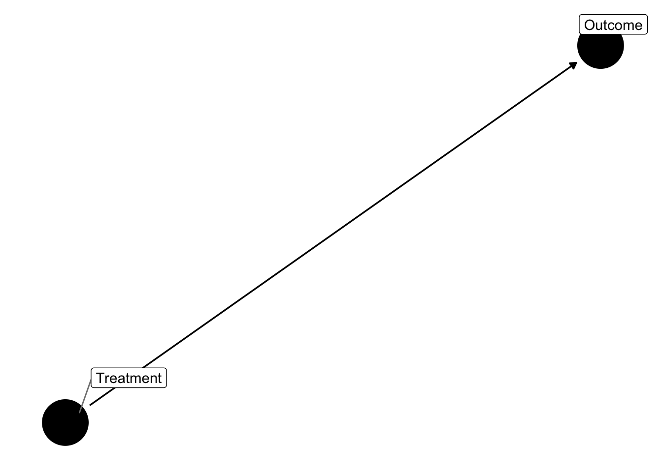
I’ll estimate the causal effect of the treatment on the outcome using a regular two-way fixed effects (TWFE) regression of the form:
\[y_{it} = \tag{1} \alpha_i + \alpha_t + \sum_{t = min + 1, t \neq -1}^{max} \gamma_i \cdot D_{it} + \epsilon\]
This is a normal event study design where we fully saturate in relative time indicators, but leave out two relative periods (following Borusyak & Jaravel (2017)), the most negative relative time indicator and the indicator for the year before treatment (t = -1). We know what the true treatment effect is here = 0.2 times the years since treatment for each post-treatment period. I will plot the true treatment effect, along with the estimates from regression (1) below:
theme_set(theme_clean() + theme(plot.background = element_blank()))

# first make a plot where log age has no impact on the outcome variable
# get var names in a vector - need to drop the most negative lag (lag_1) and
min <- min(data$rel_year, na.rm = TRUE) + 1
max <- max(data$rel_year, na.rm = TRUE)

# make string for rel time indicators
indics <- paste0(c(paste0("`lag_", seq(min, -2), "`"),
                   paste0("lag_", seq(0, max))),
                 collapse = " + ")

# make the formula we want to run
form <- as.formula(paste0("y ~ ", indics, "| unit + year | 0 | unit"))

# get true taus to merge in
true_taus <- tibble(
  time = seq(-10, 10),
  true_tau = c(rep(0, length(-10:-1)), .2*(0:10 + 1))
)

# estimate the model and make the plot
data %>%
  # generate the outcome variable
  mutate(y = unit_fe + year_fe + cumtau + error) %>%
  # run the model and tidy up
  do(broom::tidy(felm(form, data = .), conf.int = TRUE)) %>%
  filter(term != "firm_age") %>%
  # make the relative time variable and keep just what we need
  mutate(time = c(min:(-2), 0:max)) %>%
  select(time, estimate, conf.low, conf.high) %>%
  # bring back in missing indicator for t = -1
  bind_rows(tibble(
    time = -1, estimate = 0, conf.low = 0, conf.high = 0
  )) %>%
  # keep just -10 to 10
  filter(time %>% between(-10, 10)) %>%
  left_join(true_taus) %>%
  # split the error bands by pre-post
  mutate(band_groups = case_when(
    time < -1 ~ "Pre",
    time >= 0 ~ "Post",
    time == -1 ~ ""
  )) %>%
  # plot it
  ggplot(aes(x = time, y = estimate)) +
  geom_line(aes(x = time, y = true_tau, color = "True Effect"), size = 1.5, linetype = "dashed") +
  geom_ribbon(aes(ymin = conf.low, ymax = conf.high, group = band_groups),
              color = "lightgrey", alpha = 1/4) +
  geom_pointrange(aes(ymin = conf.low, ymax = conf.high, color = "Estimated Effect"),
                  show.legend = FALSE) +
  geom_hline(yintercept = 0) +
  geom_vline(xintercept = -0.5, linetype = "dashed") +
  scale_x_continuous(breaks = seq(-10, 10, by = 2)) +
  labs(x = "Relative Time", y = "Estimate") +
  scale_color_brewer(palette = 'Set1') +
  theme(legend.position = "bottom",
        legend.title = element_blank(),
        axis.title = element_text(size = 18),
        axis.text = element_text(size = 16))
Life is good, we recover the true treatment effect path. As an important aside, note that we fully saturated the time fixed effects here. What if we do what is more common in the literature and bin all year before t - 10 into a Pre variable and all years after t + 10 into a Post variable?
theme_set(theme_clean() + theme(plot.background = element_blank()))

# first make a plot where log age has no impact on the outcome variable
# get var names in a vector - need to drop the most negative lag (lag_1) and
min <- min(data$rel_year, na.rm = TRUE) + 1
max <- max(data$rel_year, na.rm = TRUE)

# make string for rel time indicators
indics <- paste0(c("Pre", "Post",
                   paste0("`lag_", seq(-10, -2), "`"),
                   paste0("lag_", seq(0, 10))),
                 collapse = " + ")

# make the formula we want to run
form <- as.formula(paste0("y ~ ", indics, "| unit + year | 0 | unit"))

# estimate the model and make the plot
data %>%
  # make pre and post variables
  mutate(Pre = if_else(!is.na(rel_year) & rel_year < 10, 1, 0),
         Post = if_else(!is.na(rel_year) & rel_year > 10, 1, 0)) %>%
  # generate the outcome variable
  mutate(y = unit_fe + year_fe + cumtau + error) %>%
  # run the model and tidy up
  do(broom::tidy(felm(form, data = .), conf.int = TRUE)) %>%
  filter(!(term %in% c("firm_age", "Pre", "Post"))) %>%
  # make the relative time variable and keep just what we need
  mutate(time = c(-10:(-2), 0:10)) %>%
  select(time, estimate, conf.low, conf.high) %>%
  # bring back in missing indicator for t = -1
  bind_rows(tibble(
    time = -1, estimate = 0, conf.low = 0, conf.high = 0
  )) %>%
  # keep just -10 to 10
  filter(time %>% between(-10, 10)) %>%
  left_join(true_taus) %>%
  # split the error bands by pre-post
  mutate(band_groups = case_when(
    time < -1 ~ "Pre",
    time >= 0 ~ "Post",
    time == -1 ~ ""
  )) %>%
  # plot it
  ggplot(aes(x = time, y = estimate)) +
  geom_line(aes(x = time, y = true_tau, color = "True Effect"), size = 1.5, linetype = "dashed") +
  geom_ribbon(aes(ymin = conf.low, ymax = conf.high, group = band_groups),
              color = "lightgrey", alpha = 1/4) +
  geom_pointrange(aes(ymin = conf.low, ymax = conf.high, color = "Estimated Effect"),
                  show.legend = FALSE) +
  geom_hline(yintercept = 0) +
  geom_vline(xintercept = -0.5, linetype = "dashed") +
  scale_x_continuous(breaks = seq(-10, 10, by = 2)) +
  labs(x = "Relative Time", y = "Estimate") +
  scale_color_brewer(palette = 'Set1') +
  theme(legend.position = "bottom",
        legend.title = element_blank(),
        axis.title = element_text(size = 18),
        axis.text = element_text(size = 16))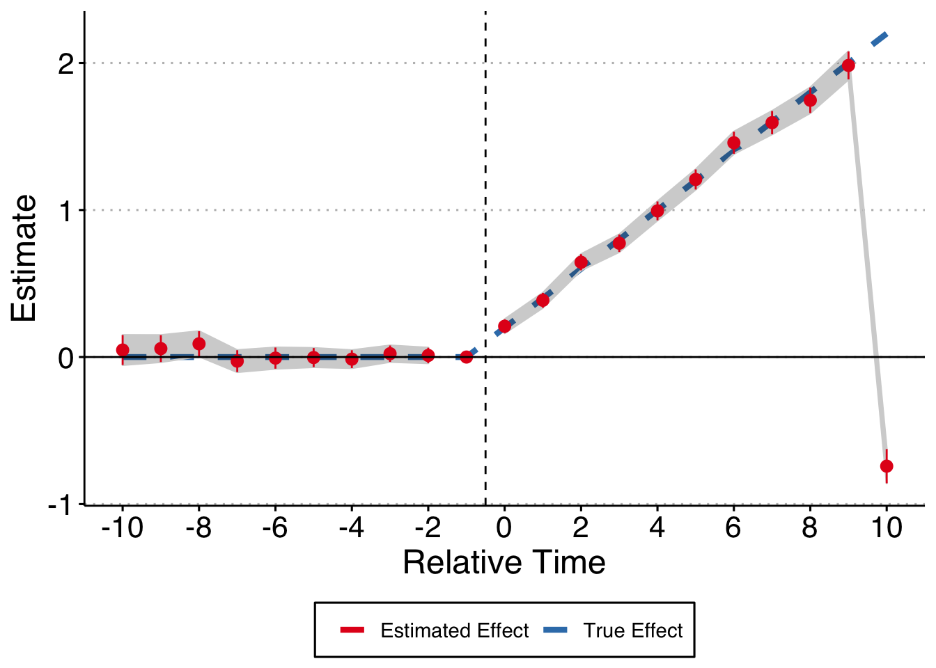
Whoops! That’s no good. Try messing around with different forms of this, either only putting in the relative time indicators (thus leaving out both Pre and Post) or dropping one or the other, and you’ll see that things get really wonky. It depends on your DGP but we should all be fully saturating the relative time indicators every time.
Moving on, what if you were to erroneously control for log age even though it isn’t related to either the outcome or the treatment? We’re still good (this should be obvious, but it’s nice to think through these relations and prove it to yourself).
theme_set(theme_clean() + theme(plot.background = element_blank()))

# make string for rel time indicators
indics <- paste0(c(paste0("`lag_", seq(min, -2), "`"),
                   paste0("lag_", seq(0, max))),
                 collapse = " + ")

# make the formula we want to run
form <- as.formula(paste0("y ~ ", indics, " + log_age | unit + year | 0 | unit"))

# estimate the model and make the plot
data %>%
  # generate the outcome variable
  mutate(y = unit_fe + year_fe + cumtau + error) %>%
  # run the model and tidy up
  do(broom::tidy(felm(form, data = .), conf.int = TRUE)) %>%
  filter(term != "log_age") %>%
  # make the relative time variable and keep just what we need
  mutate(time = c(min:(-2), 0:max)) %>%
  select(time, estimate, conf.low, conf.high) %>%
  # bring back in missing indicator for t = -1
  bind_rows(tibble(
    time = -1, estimate = 0, conf.low = 0, conf.high = 0
  )) %>%
  # keep just -10 to 10
  filter(time %>% between(-10, 10)) %>%
  left_join(true_taus) %>%
  # split the error bands by pre-post
  mutate(band_groups = case_when(
    time < -1 ~ "Pre",
    time >= 0 ~ "Post",
    time == -1 ~ ""
  )) %>%
  # plot it
  ggplot(aes(x = time, y = estimate)) +
  geom_line(aes(x = time, y = true_tau, color = "True Effect"), size = 1.5, linetype = "dashed") +
  geom_ribbon(aes(ymin = conf.low, ymax = conf.high, group = band_groups),
              color = "lightgrey", alpha = 1/4) +
  geom_pointrange(aes(ymin = conf.low, ymax = conf.high, color = "Estimated Effect"),
                  show.legend = FALSE) +
  geom_hline(yintercept = 0) +
  geom_vline(xintercept = -0.5, linetype = "dashed") +
  scale_x_continuous(breaks = seq(-10, 10, by = 2)) +
  labs(x = "Relative Time", y = "Estimate") +
  scale_color_brewer(palette = 'Set1') +
  theme(legend.position = "bottom",
        legend.title = element_blank(),
        axis.title = element_text(size = 18),
        axis.text = element_text(size = 16))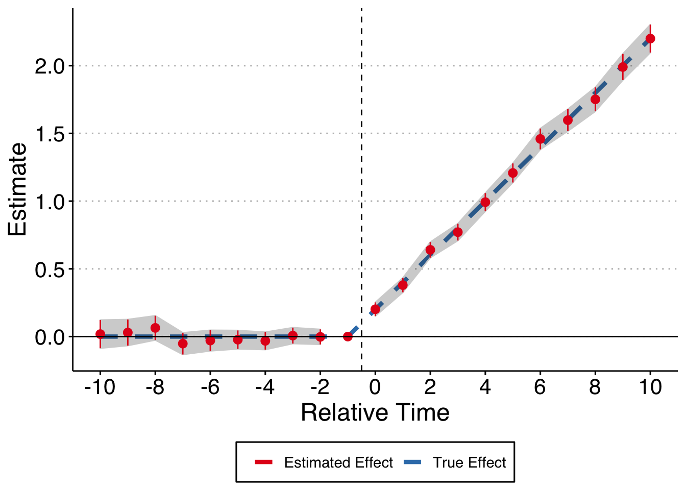
Okay, let’s start to make things more interesting. First, what if our log_age variable is associated with our outcome variable, but not with the treatment. Now I change the DGP to be:
\[y_{it} = \tag{1} \alpha_i + \alpha_t + \sum_{t = min + 1, t \neq -1}^{max} \gamma_i \cdot D_{it} - 0.85 \cdot log\_age + \epsilon\]
dagify(y ~ t,
       y ~ x,
       labels = c("y" = "Outcome",
                  "t" = "Treatment",
                  "x" = "Log of Firm Age")) %>%
  ggdag(text = FALSE, use_labels = "label") +
  theme_dag()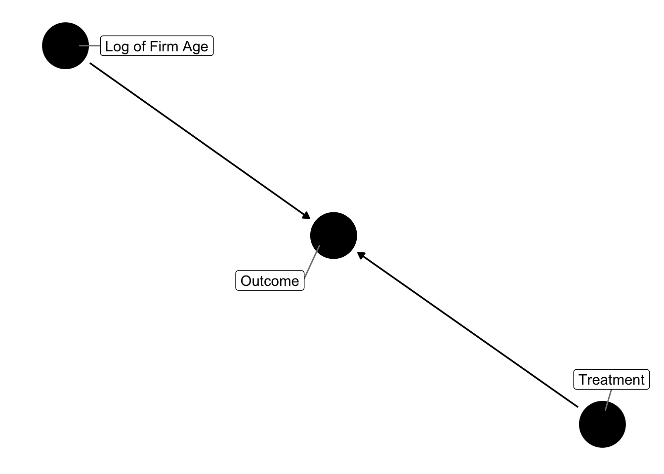
If we run the regression controlling and control for log_age, we’re good. (Note, you shouldn’t need to control for log_age here because it isn’t a confounding variable - it only impacts the outcome variable. But, there are weird time dynamics that intersect with our relative period dummies and the omitted variables - essentially firm age is associated with the relative time dummies because time only goes in one direction and so does treatment assignment. Too tired to think through the consequences here, but with this DGP you do need to control for log_age to exactly hit the estimates with TWFE).
theme_set(theme_clean() + theme(plot.background = element_blank()))

# next, assume that there is an effect on the outcome variable but no effect on the treatment outcome
# make string for rel time indicators
indics <- paste0(c(paste0("`lag_", seq(min, -2), "`"),
                   paste0("lag_", seq(0, max))),
                 collapse = " + ")

form <- as.formula(paste0("y ~ ", indics, "  + log_age| unit + year | 0 | unit"))

# estimate the model and make the plot
data %>%
  # generate the outcome variable
  mutate(y = unit_fe + year_fe + cumtau + -.85*log_age + error) %>%
  # run the model and tidy up
  do(broom::tidy(felm(form, data = .), conf.int = TRUE)) %>%
  # make the relative time variable and keep just what we need
  filter(term != "log_age") %>%
  mutate(time = c(min:(-2), 0:max)) %>%
  select(time, estimate, conf.low, conf.high) %>%
  # bring back in missing indicator for t = -1
  # bring back in missing indicator for t = -1
  bind_rows(tibble(
    time = -1, estimate = 0, conf.low = 0, conf.high = 0
  )) %>%
  # keep just -10 to 10
  filter(time %>% between(-10, 10)) %>%
  left_join(true_taus) %>%
  # split the error bands by pre-post
  mutate(band_groups = case_when(
    time < -1 ~ "Pre",
    time >= 0 ~ "Post",
    time == -1 ~ ""
  )) %>%
  # plot it
  ggplot(aes(x = time, y = estimate)) +
  geom_line(aes(x = time, y = true_tau, color = "True Effect"), size = 1.5, linetype = "dashed") +
  geom_ribbon(aes(ymin = conf.low, ymax = conf.high, group = band_groups),
              color = "lightgrey", alpha = 1/4) +
  geom_pointrange(aes(ymin = conf.low, ymax = conf.high, color = "Estimated Effect"),
                  show.legend = FALSE) +
  geom_hline(yintercept = 0) +
  geom_vline(xintercept = -0.5, linetype = "dashed") +
  scale_x_continuous(breaks = seq(-10, 10, by = 2)) +
  labs(x = "Relative Time", y = "Estimate") +
  scale_color_brewer(palette = 'Set1') +
  theme(legend.position = "bottom",
        legend.title = element_blank(),
        axis.title = element_text(size = 18),
axis.text = element_text(size = 16)) 
Finally, what if log_age is a confounding variable? That is, it impacts both the treatment and outcome variable and needs to be controlled for under causal-inference-dag-circle-drawing dogma:
dagify(y ~ t,
       y ~ x,
       t ~ x,
       labels = c("y" = "Outcome",
                  "t" = "Treatment",
                  "x" = "Log of Firm Age")) %>%
  ggdag(text = FALSE, use_labels = "label") +
  theme_dag()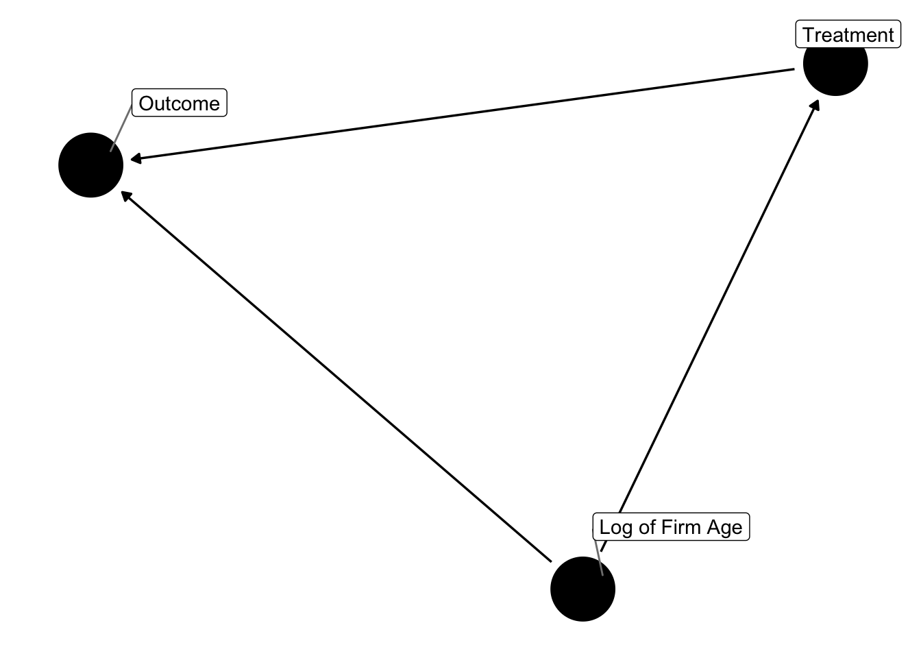
I implement this somewhat cludgely, but essentially I simulate the data in the same manner as above, but now the treatment assignment is in part determined by firm age. For each firm I get their average age in the panel and use that as an inverse weight when I randomly assign the treatment to firms (probably better ways to do this but it works). Now, not only is the estimate still valid when controlling for log_age but you in fact need to control for it to get unbiased estimates.
theme_set(theme_clean() + theme(plot.background = element_blank()))

# Now assume that the log age variable is correlated in some way with the treatment assignment decision
# in particular assume that younger firms are more likely to get targeted

# Generate data - 20,000 firms are placed in each group. Groups 3 and 4 are
# treated in 1998, Groups 1 and 2 are untreated

make_data <- function(...) {

  # Fixed Effects ------------------------------------------------
  # unit fixed effects
  unit <- tibble(
    unit = 1:20000,
    unit_fe = rnorm(20000, 0, 1)) %>%
    # make first and last year per unit, and treat year if treated
    rowwise() %>%
    mutate(first_year = sample(seq(1981, 2010), 1),
           # pull last year as a randomly selected date bw first and 2010
           last_year = if_else(first_year < 2010, sample(seq(first_year, 2010), 1),
                               as.integer(2010))) %>%
    ungroup()

  # year fixed effects
  year <- tibble(
    year = 1981:2010,
    year_fe = rnorm(30, 0, 1))

  # make panel
  data <- crossing(unit, year) %>%
    arrange(unit, year) %>%
    # keep only if year between first and last year
    rowwise() %>%
    filter(year %>% between(first_year, last_year)) %>%
    ungroup() %>%
    mutate(firm_age = year - first_year)

    # make an average age data frame
  avg_age <- data %>%
    group_by(unit) %>%
    summarize(avg_age = mean(firm_age)) %>%
    mutate(weight = 1 / (avg_age + 1))

  # sample 4,000 firms to get treatment, weighted by average age
  treated_units <- sample_n(avg_age, 4000, replace = FALSE, weight = weight) %>%
    mutate(treat = 1) %>%
    select(unit, treat)

  # merge treat back into the data
  treat_data <- data %>%
    select(unit, first_year, last_year) %>%
    distinct() %>%
    left_join(treated_units) %>%
    replace_na(list(treat = 0)) %>%
    rowwise() %>%
    mutate(treat_year = if_else(treat == 1,
                                if_else(first_year != last_year,
                                        sample(first_year:last_year, 1), as.integer(first_year)),
                                as.integer(0)))

  # merge back into main data
  data <- data %>%
    left_join(treat_data) %>%
    # make error term, treat term and log age term
    mutate(error = rnorm(nrow(.), 0, 1),
           posttreat = if_else(treat == 1 & year >= treat_year, 1, 0),
           rel_year = if_else(treat == 1, year - treat_year, as.integer(NA)),
           tau = if_else(posttreat == 1, .2, 0),
           firm_age = year - first_year,
           log_age = log(firm_age + 1)) %>%
    # make cumulative treatment effects
    group_by(unit) %>%
    mutate(cumtau = cumsum(tau)) %>%
    ungroup() %>%
    # finally, make dummy variables
    bind_cols(dummy_cols(tibble(lag = .$rel_year), select_columns = "lag",
                         ignore_na = TRUE, remove_selected_columns = TRUE)) %>%
    # replace equal to 0 for all lead lag columns
    mutate_at(vars(starts_with("lag_")), ~replace_na(., 0))
}

# make data
data2 <- make_data()

# get var names in a vector - need to drop the most negative lag (lag_1) and
min <- min(data2$rel_year, na.rm = TRUE) + 1
max <- max(data2$rel_year, na.rm = TRUE)

# make string for rel time indicators
indics <- paste0(c(paste0("`lag_", seq(min, -2), "`"),
                   paste0("lag_", seq(0, max))),
                 collapse = " + ")

# make the formula we want to run
form1 <- as.formula(paste0("y ~ ", indics, "| unit + year | 0 | unit"))
form2 <- as.formula(paste0("y ~ ", indics, " + log_age| unit + year | 0 | unit"))

# estimate the model and make the plot
data2 %>%
  # generate the outcome variable
  mutate(y = unit_fe + year_fe + cumtau + -.85*log_age + error) %>%
  # run the model and tidy up
  do(bind_rows(
    broom::tidy(felm(form1, data = .), conf.int = TRUE) %>% mutate(mod = "No Control Log Age"),
    broom::tidy(felm(form2, data = .), conf.int = TRUE) %>% mutate(mod = "Control Log Age"))) %>%
  # make the relative time variable and keep just what we need
  filter(term != "log_age") %>%
  mutate(time = rep(c(min:(-2), 0:max), 2)) %>%
  select(time, estimate, conf.low, conf.high, mod) %>%
  # bring back in missing indicator for t = -1
  bind_rows(tibble(
    time = rep(-1, 2), estimate = rep(0, 2), conf.low = rep(0, 2),
    conf.high = rep(0, 2), mod = c("No Control Log Age", "Control Log Age")
  )) %>%
  # keep just -10 to 10
  filter(time %>% between(-10, 10)) %>%
  left_join(true_taus) %>%
  # split the error bands by pre-post
  mutate(band_groups = case_when(
    time < -1 ~ "Pre",
    time >= 0 ~ "Post",
    time == -1 ~ ""
  )) %>%
  # plot it
  ggplot(aes(x = time, y = estimate)) +
  geom_line(aes(x = time, y = true_tau, color = "True Effect"), size = 1.5, linetype = "dashed") +
  geom_ribbon(aes(ymin = conf.low, ymax = conf.high, group = band_groups),
              color = "lightgrey", alpha = 1/4) +
  geom_pointrange(aes(ymin = conf.low, ymax = conf.high, color = "Estimated Effect"),
                  show.legend = FALSE) +
  geom_hline(yintercept = 0) +
  geom_vline(xintercept = -0.5, linetype = "dashed") +
  scale_x_continuous(breaks = seq(-10, 10, by = 2)) +
  labs(x = "Relative Time", y = "Estimate") +
  scale_color_brewer(palette = 'Set1') +
  theme(legend.position = "bottom",
        legend.title = element_blank(),
        axis.title = element_text(size = 18),
        axis.text = element_text(size = 16),
        panel.spacing = unit(2, "lines")) +
  facet_wrap(~mod)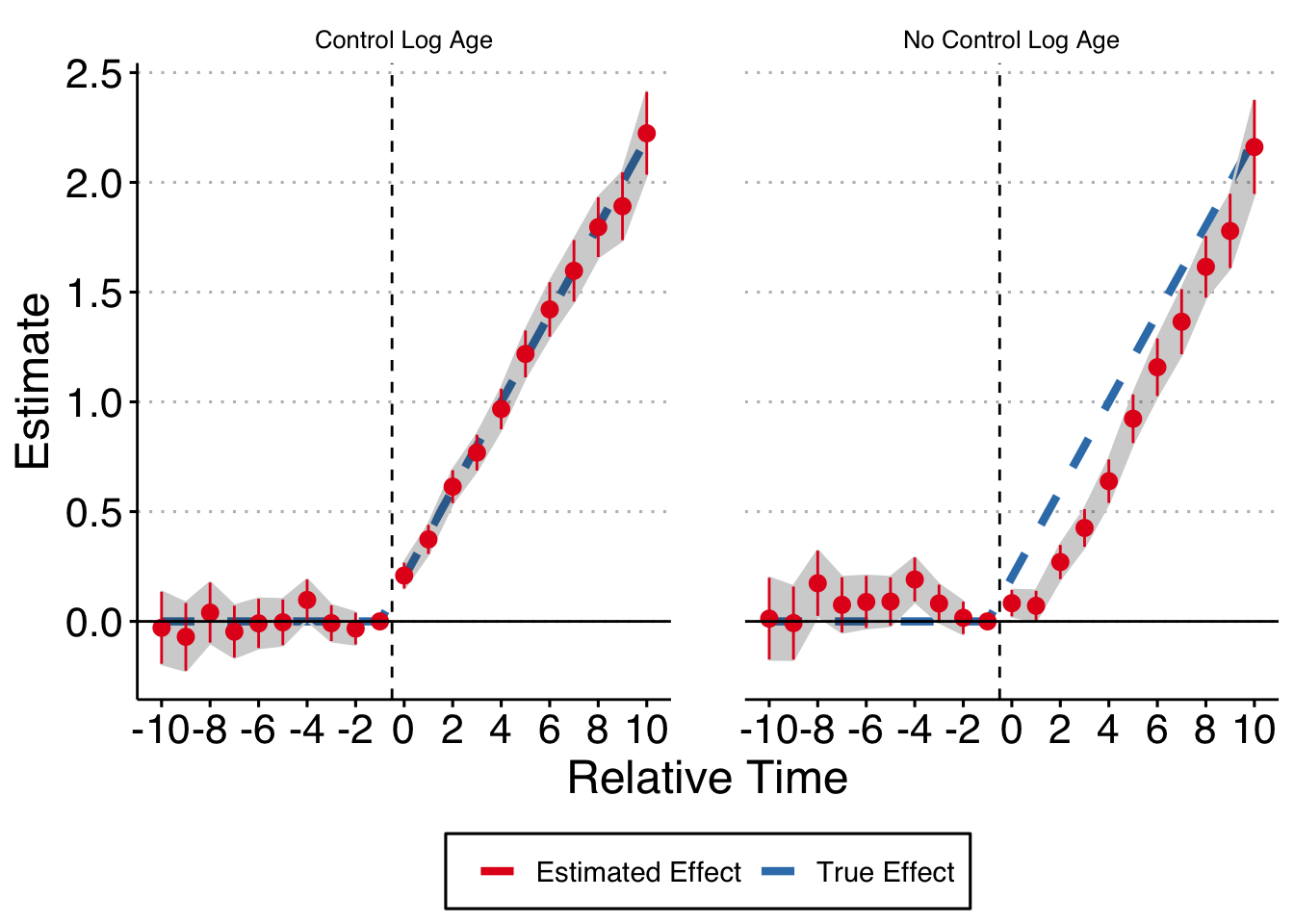
In conclusion, at least in this very straightforward example, you do need to control for the log of firm age, even though firm age itself is collinear with the fixed effects structure. Mea culpa.